The J-curve effect in trade balance illustrates how a country's trade deficit worsens initially after a currency depreciation before improving over time. When a domestic currency depreciates, the price of imported goods rises, leading to an immediate increase in the trade deficit as import volumes remain relatively stable. Over time, consumers adjust to higher prices by reducing imports, and exports become more competitive, causing the trade balance to improve and eventually surpass the initial deficit level. This phenomenon is often observed in economies with significant trade exposure and price inelastic demand for imports in the short run. For example, following a sharp depreciation of the British pound during the 1990s, the United Kingdom's trade deficit initially expanded before narrowing as export volumes increased. The J-curve effect reflects the lagged response of trade volumes to price changes, making it a critical concept for policymakers analyzing the impact of exchange rate fluctuations on trade balances.
Table of Comparison
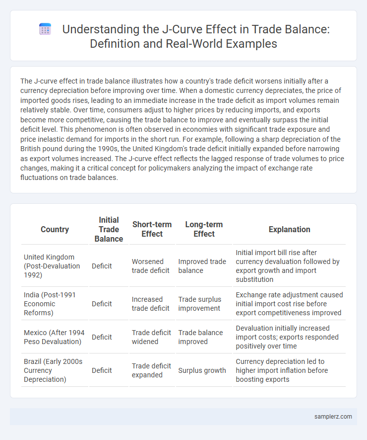
| Country | Initial Trade Balance | Short-term Effect | Long-term Effect | Explanation |
|---|---|---|---|---|
| United Kingdom (Post-Devaluation 1992) | Deficit | Worsened trade deficit | Improved trade balance | Initial import bill rise after currency devaluation followed by export growth and import substitution |
| India (Post-1991 Economic Reforms) | Deficit | Increased trade deficit | Trade surplus improvement | Exchange rate adjustment caused initial import cost rise before export competitiveness improved |
| Mexico (After 1994 Peso Devaluation) | Deficit | Trade deficit widened | Trade balance improved | Devaluation initially increased import costs; exports responded positively over time |
| Brazil (Early 2000s Currency Depreciation) | Deficit | Trade deficit expanded | Surplus growth | Currency depreciation led to higher import inflation before boosting exports |
Understanding the J-Curve Effect in Trade Balance
The J-Curve effect in trade balance occurs when a country's trade deficit initially worsens following a depreciation of its currency due to higher import prices and existing contract obligations. Over time, exports become more competitive internationally, leading to increased export volumes and improved trade balance, creating the characteristic upward curve resembling the letter "J." Empirical studies on countries like the United Kingdom and Turkey demonstrate this dynamic, highlighting the delayed positive adjustment in trade balance after currency depreciation.
Key Phases of the J-Curve Phenomenon
The J-curve phenomenon in trade balance illustrates how a country's trade deficit initially worsens following a currency depreciation due to higher import prices and contracts set in previous exchange rates. Over time, the volume effect emerges, as exports become more competitive and import demand declines, improving the trade balance. This key phase shift typically occurs after a lag period as contracts adjust, consumer behavior changes, and export growth gains momentum, ultimately resulting in a trade surplus recovery reflected in the upward curve of the J-curve.
Real-World Instances of the J-Curve in Trade
The J-curve effect in trade balance is prominently observed when a currency depreciates, initially worsening the trade deficit due to higher import costs before improving as exports become more competitive, as seen in the United Kingdom after the 1992 Black Wednesday currency devaluation. Another real-world example includes Turkey's trade balance following its 2018 currency crisis, where the lira depreciation initially expanded the deficit before exports gained momentum. These instances illustrate how exchange rate adjustments can temporally disrupt trade flows before fostering a positive shift in trade balances.
Currency Depreciation and Its Impact on Trade Balance
Currency depreciation initially worsens the trade balance due to higher import costs and unchanged export volumes, as observed in countries like Turkey after the 2018 lira depreciation. Over time, exports become more competitive globally, leading to increased export volumes and improved trade balance, a phenomenon evident in the J-curve effect during the post-depreciation period. Empirical studies show that the J-curve impact varies with the elasticity of demand for exports and imports, influencing the duration and magnitude of trade balance adjustments.
Case Study: UK Pound Depreciation and the J-Curve
The UK pound depreciation in 2016 exemplifies the J-curve effect in trade balance, where the initial impact caused a worsening deficit due to higher import costs before export volume increased. Over the subsequent quarters, British exports became more competitive internationally, improving the trade balance as demand rose and the currency's effects materialized. This case highlights how exchange rate adjustments influence trade dynamics with a lag, reflecting the J-curve phenomenon in economic analysis.
Japan’s Yen Devaluation: A J-Curve Example
Japan's yen devaluation in the early 1990s exemplifies the J-curve effect in trade balance, where the initial impact showed a worsening deficit due to higher import costs. Over time, as Japanese exports became more competitive internationally, the trade balance improved significantly. This phenomenon highlights the lag between exchange rate adjustments and their positive effect on trade surplus growth.
Emerging Markets Experiencing the J-Curve
Emerging markets often experience the J-curve effect in their trade balance following currency depreciation, where initial trade deficits worsen due to contract rigidities and higher import costs. Over time, increased export competitiveness and substitution of imports lead to an improvement in the trade balance, reflecting the upward slope of the J-curve. Countries like India and Brazil have demonstrated this phenomenon during currency adjustments, showcasing the delayed positive impact on their trade accounts.
Policy Responses to J-Curve Trade Deficits
Policy responses to J-curve trade deficits often include currency stabilization measures and export promotion initiatives to accelerate the recovery of trade balances after initial deterioration. Governments may implement targeted subsidies, improve infrastructure, and negotiate trade agreements to boost competitiveness and reduce import dependency. Monetary policies aimed at controlling inflation and interest rates can further support the adjustment process by influencing exchange rates and trade dynamics.
Long-Term Trade Balance Adjustments after Currency Shocks
The J-curve effect illustrates how a country's trade balance initially worsens following a currency depreciation due to higher import costs before improving as export volumes increase over time. Empirical studies show that after a currency shock, the trade balance often takes 12 to 24 months to adjust positively, reflecting delayed responses in contract renegotiations and export competitiveness. Long-term adjustments highlight the importance of price elasticity of demand and supply chain rigidities in the gradual recovery of trade balances.
Lessons Learned from Historical J-Curve Episodes
Historical J-curve episodes reveal that initial trade deficits often worsen following currency depreciation due to price and contract rigidities, before improving as volumes adjust. Key lessons emphasize the importance of elastic demand for imports and exports, alongside timely policy interventions to support adjustment processes. Empirical evidence from countries like the UK and Argentina highlights that recovery in trade balance depends on structural economic factors and external market conditions.
example of J-curve in trade balance Infographic