The Phillips curve illustrates the inverse relationship between unemployment and inflation rates in an economy. When unemployment decreases, inflation tends to rise due to increased wage demands as firms compete for a smaller labor pool. Historical data from the 1960s in the United States showed a clear trade-off where low unemployment corresponded with higher inflation levels. In periods of economic expansion, the Phillips curve indicates tighter labor markets, pushing wages and prices upward. Central banks monitor this relationship to balance monetary policies aimed at controlling inflation without causing excessive unemployment. Recent studies suggest that the Phillips curve may have flattened, meaning changes in unemployment have a smaller impact on inflation than in past decades.
Table of Comparison
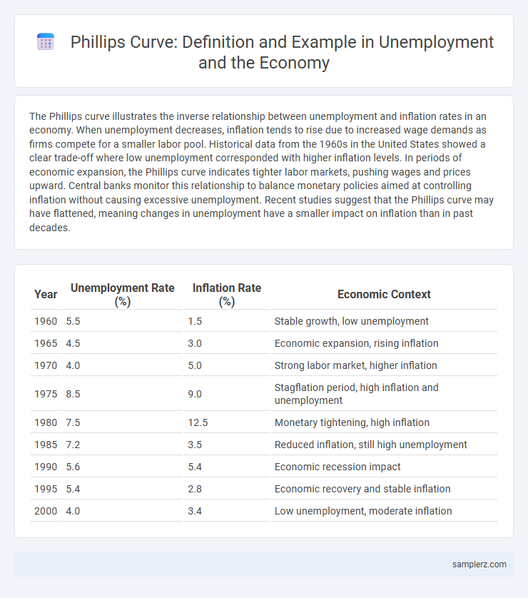
| Year | Unemployment Rate (%) | Inflation Rate (%) | Economic Context |
|---|---|---|---|
| 1960 | 5.5 | 1.5 | Stable growth, low unemployment |
| 1965 | 4.5 | 3.0 | Economic expansion, rising inflation |
| 1970 | 4.0 | 5.0 | Strong labor market, higher inflation |
| 1975 | 8.5 | 9.0 | Stagflation period, high inflation and unemployment |
| 1980 | 7.5 | 12.5 | Monetary tightening, high inflation |
| 1985 | 7.2 | 3.5 | Reduced inflation, still high unemployment |
| 1990 | 5.6 | 5.4 | Economic recession impact |
| 1995 | 5.4 | 2.8 | Economic recovery and stable inflation |
| 2000 | 4.0 | 3.4 | Low unemployment, moderate inflation |
Understanding the Phillips Curve: Definition and Economic Significance
The Phillips Curve illustrates the inverse relationship between unemployment and inflation, showing that lower unemployment rates often coincide with higher inflation. This economic model helps policymakers anticipate inflationary pressures as labor markets tighten, guiding decisions on monetary policy. Understanding this curve is crucial for balancing employment goals with price stability in macroeconomic management.
The Phillips Curve Explained Through Unemployment Examples
The Phillips Curve illustrates the inverse relationship between unemployment and inflation, showing that low unemployment rates often lead to higher wage inflation as labor demand rises. For example, during periods of near full employment, such as the late 1960s in the United States, businesses compete for scarce labor, driving wages and prices upward. Understanding this dynamic helps policymakers balance inflation control with employment goals in economic planning.
Historical Case Studies Illustrating the Phillips Curve
The 1960s United States economy exemplifies the Phillips curve, where low unemployment rates around 3.5% coincided with rising inflation nearing 5%, highlighting the inverse relationship between wage inflation and joblessness. The United Kingdom during the same period displayed similar trends, with unemployment dropping below 2% while inflation surged above 6%, reinforcing the trade-off concept. Historical case studies from these economies provide empirical evidence supporting the Phillips curve model in macroeconomic policy analysis.
Real-World Evidence of the Phillips Curve in Labor Markets
Empirical studies of the Phillips curve demonstrate a negative relationship between unemployment rates and wage inflation across various labor markets, indicating that lower unemployment levels often drive higher wage growth due to increased bargaining power of workers. For instance, during the late 1990s in the United States, declining unemployment rates corresponded with rising nominal wages and increased labor market tightness, reinforcing the Phillips curve's theoretical expectations. Recent data from Eurozone countries also reveal that as unemployment falls, inflationary pressures on wages intensify, confirming the curve's relevance in contemporary economic analysis.
How Wage Inflation Correlates with Unemployment: Classic Examples
The Phillips curve illustrates an inverse relationship between wage inflation and unemployment, demonstrated by periods such as the 1960s U.S. economy where low unemployment rates around 3-4% corresponded with rising wage inflation exceeding 5%. During times of tight labor markets, employer competition for scarce workers drives wages upward, as observed in post-World War II economies. Conversely, high unemployment levels above 8% typically suppress wage growth, reflecting diminished bargaining power among workers.
The 1970s Stagflation: A Turning Point for the Phillips Curve
The 1970s stagflation challenged the traditional Phillips curve by demonstrating the simultaneous rise of inflation and unemployment, contradicting the expected inverse relationship. During this period, supply shocks, such as the 1973 oil crisis, led to cost-push inflation while unemployment rates remained high, exposing limitations in the Phillips curve model. This economic anomaly prompted revisions in macroeconomic theory, incorporating expectations and supply-side factors to better explain the dynamics between inflation and unemployment.
Recent Phillips Curve Trends and Unemployment Rates
Recent Phillips Curve trends illustrate a weakened inverse relationship between unemployment rates and inflation, as observed in advanced economies since the late 2010s. Despite fluctuating unemployment rates influenced by events like the COVID-19 pandemic, inflation has not consistently accelerated, challenging traditional Phillips Curve predictions. Economists now emphasize factors such as global supply chain disruptions and shifting labor market dynamics to explain these deviations.
Phillips Curve Breakdown: When Unemployment and Inflation Disconnect
The Phillips Curve traditionally illustrates an inverse relationship between unemployment and inflation, suggesting lower unemployment drives higher inflation. However, during periods like the 1970s stagflation, this relationship broke down as high unemployment and high inflation occurred simultaneously, challenging the model's predictive reliability. Modern economic analysis attributes the Phillips Curve breakdown to factors such as supply shocks and inflation expectations becoming unanchored.
Central Bank Policies and Phillips Curve Examples in Unemployment
Central bank policies significantly influence the Phillips curve by managing inflation and unemployment trade-offs through interest rate adjustments. For example, during periods of expansionary monetary policy, lowering interest rates can reduce unemployment but may increase inflation, as demonstrated in the 1960s U.S. economy. Conversely, contractionary policies aimed at controlling inflation often result in higher unemployment, reflecting the Phillips curve dynamics observed in the 1970s stagflation period.
The Future of the Phillips Curve: Lessons from Recent Unemployment Data
Recent unemployment data challenges the traditional Phillips curve, revealing a weaker inverse relationship between inflation and unemployment in advanced economies. Low unemployment rates have not triggered expected inflation spikes, suggesting evolving labor market dynamics and the influence of global factors. Central banks must reconsider monetary policies as the Phillips curve's predictive power diminishes in forecasting inflation trends.
example of Phillips curve in unemployment Infographic