The J-curve effect in trade illustrates how a country's trade balance initially worsens after a currency depreciation before improving over time. When a domestic currency loses value, import costs rise, causing the trade deficit to expand temporarily. Over time, exports become more competitive globally, leading to increased export volumes and an eventual improvement in the trade balance. Data from countries like the United Kingdom following the 1992 Sterling devaluation exemplify this phenomenon. The trade deficit initially deepened as import prices surged, but subsequent export growth reversed the trend. This pattern confirms the J-curve's relevance in analyzing short-term versus long-term trade balance responses to exchange rate adjustments.
Table of Comparison
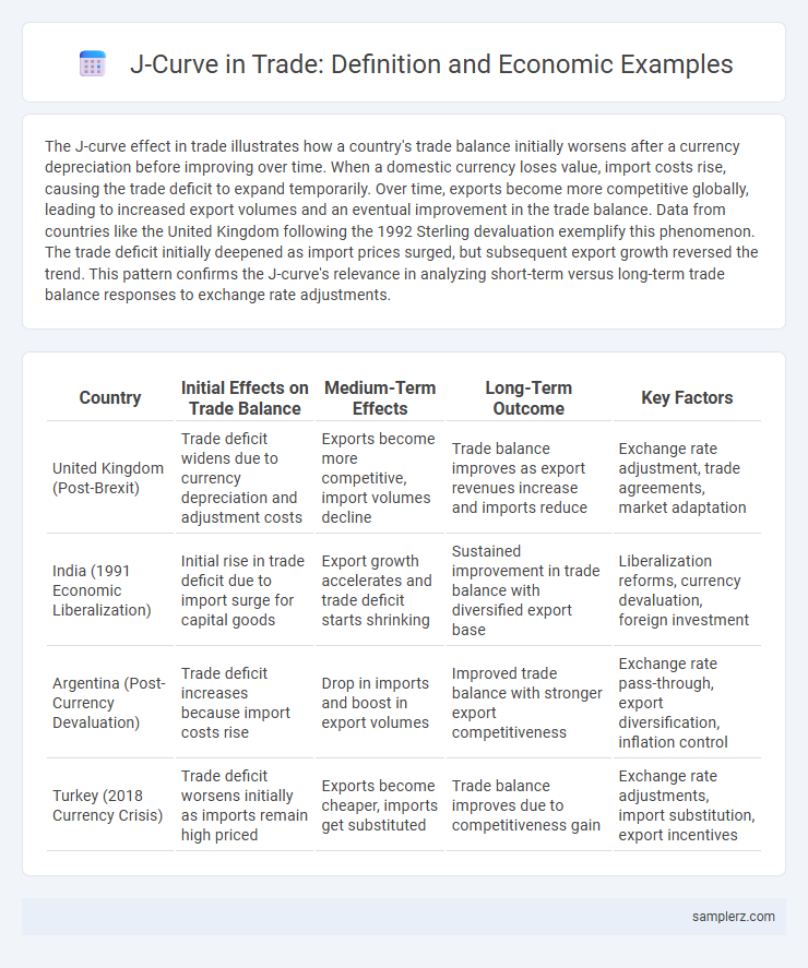
| Country | Initial Effects on Trade Balance | Medium-Term Effects | Long-Term Outcome | Key Factors |
|---|---|---|---|---|
| United Kingdom (Post-Brexit) | Trade deficit widens due to currency depreciation and adjustment costs | Exports become more competitive, import volumes decline | Trade balance improves as export revenues increase and imports reduce | Exchange rate adjustment, trade agreements, market adaptation |
| India (1991 Economic Liberalization) | Initial rise in trade deficit due to import surge for capital goods | Export growth accelerates and trade deficit starts shrinking | Sustained improvement in trade balance with diversified export base | Liberalization reforms, currency devaluation, foreign investment |
| Argentina (Post-Currency Devaluation) | Trade deficit increases because import costs rise | Drop in imports and boost in export volumes | Improved trade balance with stronger export competitiveness | Exchange rate pass-through, export diversification, inflation control |
| Turkey (2018 Currency Crisis) | Trade deficit worsens initially as imports remain high priced | Exports become cheaper, imports get substituted | Trade balance improves due to competitiveness gain | Exchange rate adjustments, import substitution, export incentives |
Understanding the J-Curve Effect in Trade
The J-Curve effect in trade illustrates how a country's trade balance initially worsens following a currency depreciation due to higher import costs before improving as export volumes increase. This phenomenon occurs because short-term contracts and price inelasticity delay the positive impact of cheaper exports on trade balance. Over time, the enhanced competitiveness of domestic goods boosts export demand, leading to a recovery and eventual improvement in the trade deficit.
Historical Examples of the J-Curve in International Trade
The historical J-Curve in international trade is exemplified by Japan's post-World War II economic recovery, where initial trade deficits worsened before significant surpluses emerged due to export-led industrial growth. Another notable instance occurred in Germany after reunification in 1990, where the integration of East Germany initially increased imports and trade deficits before export competitiveness improved, reversing the trend. These cases highlight the typical J-shaped trajectory as economies adjust trade balances following major structural changes.
The J-Curve Phenomenon: Currency Depreciation and Trade Balance
Currency depreciation initially worsens a country's trade balance due to higher import costs and rigid short-term contracts. Over time, export volumes increase as domestic goods become more competitively priced, leading to improved trade balances. This dynamic process exemplifies the J-curve phenomenon, where trade deficits deepen before recovering and transitioning into surpluses.
Case Study: UK’s J-Curve Experience after Currency Devaluation
The UK's J-curve experience following the 1992 currency devaluation illustrates a short-term trade deficit deterioration before improvement. Initial import costs rose due to a weaker pound, exacerbating the trade balance, but over time, export volumes increased and import demand declined. This case study highlights the delayed positive impact of devaluation on trade balance, consistent with the J-curve hypothesis in international economics.
The J-Curve in Emerging Market Economies
Emerging market economies often experience a J-curve effect in trade when currency depreciation initially worsens the trade balance due to higher import costs and existing contract rigidities. Over time, as export volumes increase and import demand adjusts, the trade balance improves significantly, reflecting the typical J-shaped recovery. This phenomenon is prominently observed in countries like India and Brazil during periods of currency realignment and trade liberalization.
Short-term vs. Long-term Impacts of the J-Curve on Trade
The J-curve effect in trade illustrates a country's trade balance initially deteriorating after currency depreciation due to higher import costs and unchanged export volumes. Over time, exports become more competitive and import demand adjusts, leading to an improved trade balance and positive long-term economic growth. This dynamic highlights the short-term trade deficit increase versus the long-term gain in export strength and trade balance recovery.
The Role of Price Elasticity in the J-Curve Effect
Price elasticity plays a crucial role in the J-curve effect by influencing how the volume of imports and exports responds to exchange rate fluctuations. When a currency depreciates, low initial price elasticity causes trade deficits to worsen before improving, as quantities demanded adjust sluggishly. Over time, higher price elasticity increases export volumes and reduces imports, resulting in an overall improvement in the trade balance consistent with the J-curve pattern.
J-Curve Examples: Developed vs. Developing Countries
The J-curve effect in trade illustrates how a country's trade balance initially worsens after a currency depreciation before improving over time as export volumes increase. Developed countries, like the United States, often show a pronounced J-curve due to diversified economies and strong export demand resilience. Developing countries, such as India, may experience a delayed or less distinct J-curve impact because of structural trade dependencies and lower price elasticity of exports and imports.
Policy Implications of the J-Curve in Trade Adjustment
The J-curve in trade adjustment illustrates how a country's trade balance initially worsens following a depreciation of its currency before improving over time as export volumes increase. Policy implications emphasize the need for short-term support measures, such as fiscal stimulus or targeted subsidies, to cushion the temporary negative effects on import costs and inflation. Effective exchange rate management and structural reforms enhance the long-term benefits by improving export competitiveness and facilitating smoother trade transitions.
Limitations of the J-Curve Theory in Real-World Trade Scenarios
The J-Curve theory illustrates how a country's trade balance initially worsens following a currency devaluation before improving over time, but its application faces several limitations in real-world trade scenarios. Factors such as price elasticity of demand, time lags in contract adjustments, and varying economic conditions across trading partners often distort the predicted trajectory, preventing a smooth J-shaped recovery. Empirical evidence shows that some countries experience prolonged trade deficits or fail to achieve the expected improvement, highlighting the theory's oversimplification of complex international trade dynamics.
example of J-curve in trade Infographic