The Phillips curve illustrates the inverse relationship between unemployment rates and inflation within an economy. For example, during the 1960s in the United States, low unemployment levels corresponded with rising inflation, highlighting the trade-off faced by policymakers. This period demonstrated how inflation tended to accelerate when the job market tightened, reducing unemployment below its natural rate. Recent data from emerging markets also reflect the Phillips curve dynamics, where inflation surged as unemployment decreased during economic expansions. Central banks monitor this relationship to calibrate monetary policy, aiming to balance inflation targets with employment goals. Understanding the Phillips curve aids in predicting inflationary pressures linked to labor market fluctuations.
Table of Comparison
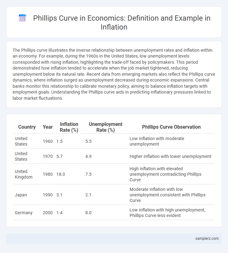
| Country | Year | Inflation Rate (%) | Unemployment Rate (%) | Phillips Curve Observation |
|---|---|---|---|---|
| United States | 1960 | 1.5 | 5.5 | Low inflation with moderate unemployment |
| United States | 1970 | 5.7 | 4.9 | Higher inflation with lower unemployment |
| United Kingdom | 1980 | 18.0 | 7.5 | High inflation with elevated unemployment contradicting Phillips Curve |
| Japan | 1990 | 3.1 | 2.1 | Moderate inflation with low unemployment consistent with Phillips Curve |
| Germany | 2000 | 1.4 | 8.0 | Low inflation with high unemployment, Phillips Curve less evident |
Real-World Application of the Phillips Curve in Inflation Analysis
The Phillips curve illustrates the inverse relationship between inflation and unemployment, exemplified by the 1960s U.S. economy where low unemployment coincided with rising inflation rates. Policymakers use this model to anticipate inflationary pressures when unemployment falls below its natural rate, adjusting monetary policy accordingly. Contemporary analyses incorporate expectations-augmented Phillips curves to address inflation persistence despite varying unemployment levels.
Case Study: The Phillips Curve During the 1970s Stagflation
The Phillips Curve, predicting an inverse relationship between inflation and unemployment, broke down during the 1970s stagflation when both inflation and unemployment surged simultaneously in many developed economies. This period highlighted the limitations of traditional Phillips Curve theory as supply shocks, such as the 1973 oil crisis, disrupted the trade-off and caused stagflation. Economists later integrated expectations and supply-side factors into models to better explain inflation and unemployment dynamics during periods of stagflation.
How Central Banks Use the Phillips Curve to Predict Inflation
Central banks utilize the Phillips Curve to estimate the trade-off between unemployment and inflation, adjusting monetary policy to stabilize prices and support employment levels. By analyzing historical data linking wage growth with labor market tightness, policymakers anticipate inflationary pressures during periods of low unemployment. This predictive use helps guide interest rate decisions to prevent overheating or recession in the economy.
Phillips Curve Evidence in Emerging Market Economies
Emerging market economies exhibit a discernible Phillips curve relationship where lower unemployment rates often coincide with higher inflation rates due to wage pressures and demand-pull factors. Empirical studies in countries like Brazil, India, and South Africa reveal that inflation expectations and supply-side shocks can modify the traditional Phillips curve dynamics. These findings underscore the importance of considering inflation inertia and structural constraints in monetary policy formulation within emerging markets.
Historical Inflation Trends Explained by the Phillips Curve
The Phillips curve illustrates the inverse relationship between unemployment and inflation, as seen during the 1960s when low unemployment in the U.S. corresponded with rising inflation rates. Historical data reveals that periods of tight labor markets typically drive wage increases, fueling higher consumer prices and accelerating inflation. This dynamic helps explain inflationary trends during economic expansions before supply shocks and expectations adjustments altered the curve's predictive power.
Impact of Supply Shocks on the Phillips Curve Relationship
Supply shocks, such as sudden increases in oil prices, shift the Phillips curve upward by causing higher inflation without corresponding decreases in unemployment. This disruption weakens the traditional inverse relationship between inflation and unemployment embedded in the Phillips curve. Policymakers must adjust expectations and consider supply-side factors to accurately interpret inflation dynamics during such shocks.
Phillips Curve Analysis: US Economy in the Post-2008 Era
The Phillips Curve in the post-2008 US economy reveals a weakened inverse relationship between unemployment and inflation, as low unemployment rates did not trigger significant wage or price increases. Federal Reserve data highlight periods where inflation remained subdued despite near full employment, challenging traditional Phillips Curve predictions. This shift underscores structural changes such as globalization, labor market slack, and anchored inflation expectations influencing the US inflation-unemployment dynamics.
The Role of Expectations in Phillips Curve Inflation Examples
The Phillips curve demonstrates the inverse relationship between unemployment and inflation, with expectations playing a critical role in its dynamics. When inflation expectations rise, workers demand higher wages to keep up with anticipated price increases, causing the short-run Phillips curve to shift upward and leading to higher actual inflation without significant changes in unemployment. Empirical evidence from the 1970s stagflation period highlights how adaptive expectations contributed to a breakdown of the traditional Phillips curve relationship, emphasizing the importance of inflation expectations in shaping inflation outcomes.
Comparing Phillips Curve Performance across Developed Economies
The Phillips Curve illustrates the inverse relationship between inflation and unemployment, yet its accuracy varies across developed economies such as the United States, Germany, and Japan. In the U.S., the curve remained relatively stable during the 1960s but has flattened since the 2008 financial crisis, reflecting weaker inflationary responses to labor market tightening. Germany and Japan exhibit even flatter Phillips Curves due to factors like labor market rigidities and aging populations, which dampen wage pressures despite low unemployment rates.
Inflation Targeting and the Phillips Curve in Practice
Inflation targeting, a monetary policy strategy central banks use to maintain price stability, directly interacts with the Phillips curve by influencing inflation expectations and unemployment rates. Empirical evidence shows that strict inflation targeting can flatten the Phillips curve, reducing the trade-off between inflation and unemployment over time. Central banks like the Reserve Bank of New Zealand have demonstrated that credible inflation targeting stabilizes inflation without causing significant unemployment fluctuations, exemplifying the Phillips curve's practical application in modern economic policy.
example of Phillips curve in inflation Infographic