The J-curve effect in exchange rates occurs when a country's trade balance initially worsens following a depreciation of its currency before improving over time. This phenomenon is attributed to the delayed response of import and export volumes to changes in exchange rates, where the cost of imports rises immediately while export volumes take time to increase. Empirical data from countries such as the United Kingdom post-Brexit show a clear J-curve pattern in the months after the pound's depreciation. In economic analysis, the J-curve highlights the dynamic relationship between currency depreciation and trade balance adjustments. Exporters eventually benefit as their goods become cheaper and more competitive internationally, which boosts export volumes. Data from the International Monetary Fund reveals that emerging markets frequently demonstrate J-curve effects after currency devaluation, reflecting initial trade deficits followed by gradual improvements.
Table of Comparison
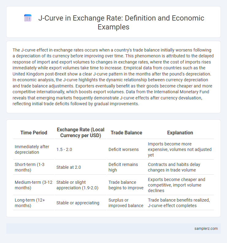
| Time Period | Exchange Rate (Local Currency per USD) | Trade Balance | Explanation |
|---|---|---|---|
| Immediately after depreciation | 1.5 - 2.0 | Deficit worsens | Imports become more expensive, volumes not adjusted yet |
| Short-term (1-3 months) | Stable at 2.0 | Deficit remains high | Contracts and habits delay changes in trade volume |
| Medium-term (3-12 months) | Stable or slight appreciation (1.9-2.0) | Trade balance begins to improve | Exports become cheaper and competitive, import volume declines |
| Long-term (12+ months) | Stable or appreciating | Surplus or improved balance | Trade balance benefits realized, J-curve effect completes |
Understanding the J-Curve Effect in Exchange Rate Economics
The J-curve effect in exchange rate economics illustrates how a country's trade balance initially worsens following a currency depreciation before improving over time. This phenomenon occurs because prices of imports rise immediately while export volumes take time to respond to more competitive pricing. Empirical studies show that the trade balance often shifts positively after a lag period as contracts renegotiate and demand elasticity adjusts, confirming the typical J-shaped trajectory.
Key Examples of the J-Curve in Historical Exchange Rate Movements
The J-curve effect is evident in the early 1980s when the US dollar appreciated sharply against major currencies, initially worsening the trade balance before improving it as export competitiveness returned. Another key example is the British pound's depreciation after the 2008 financial crisis, where the trade deficit deepened before gradually narrowing due to increased export volumes. These historical movements highlight how exchange rate adjustments can temporarily exacerbate trade imbalances before producing favorable outcomes.
The J-Curve Phenomenon: Impact on Trade Balances
The J-Curve phenomenon illustrates how a country's trade balance initially worsens following a currency depreciation due to price effects on existing contracts and import costs. Over time, quantity adjustments lead to improved export competitiveness, eventually enhancing the trade balance as demand for cheaper domestic goods rises. Empirical studies of exchange rate fluctuations in economies like Turkey and Japan confirm the delayed positive impact on trade balances characteristic of the J-Curve effect.
Case Study: The UK Pound’s J-Curve After the 1992 ERM Crisis
The UK Pound experienced a classic J-curve effect following the 1992 Exchange Rate Mechanism (ERM) crisis, where its initial sharp depreciation led to a worsening trade balance before eventual improvement. After the pound was forced out of the ERM and devalued, export competitiveness increased, boosting trade surpluses within months despite early rising import costs. This case exemplifies how currency devaluation temporarily exacerbates trade deficits before generating enhanced export-driven economic recovery.
The J-Curve Effect in Emerging Market Currency Devaluations
The J-curve effect occurs when an emerging market's currency devaluation initially worsens its trade balance before improving it over time due to delayed adjustments in export volumes and import prices. Empirical studies reveal that countries like Turkey and South Africa experience a negative trade deficit impact within the first few quarters post-devaluation, followed by a gradual recovery as competitiveness improves. Understanding this dynamic is crucial for policymakers to anticipate short-term economic strain while targeting long-term export growth.
How the J-Curve Explains Delayed Trade Balance Improvement
The J-Curve effect in exchange rates illustrates how a country's trade balance initially worsens after a currency depreciation before improving over time. This delay occurs because import prices rise immediately, increasing the trade deficit, while export volumes take longer to respond due to contract lags and adjustment costs. Over the medium term, export competitiveness improves and import demand falls, leading to a gradual recovery and eventual enhancement of the trade balance.
Japan’s Yen Devaluation: A Modern J-Curve Example
Japan's Yen devaluation in the 2010s exemplifies the J-curve effect, where the immediate aftermath showed a worsening trade balance due to higher import costs. Over time, improved export competitiveness led to increased export volumes, reversing the deficit and enhancing trade balance outcomes. This dynamic illustrates how currency depreciation initially causes trade deficits before stimulating export growth and economic recovery.
The Role of Elasticities in the J-Curve of Exchange Rates
The J-curve effect in exchange rates demonstrates how a currency depreciation initially worsens the trade balance before improving it, largely due to the price elasticities of exports and imports. When demand for imports and exports is inelastic, quantities traded change little immediately, causing the trade deficit to widen despite lower currency value. Over time, as elasticities adjust and consumers respond to price changes, export volumes increase and import volumes decrease, leading to an improved trade balance consistent with the J-curve hypothesis.
Policy Implications of the J-Curve in Currency Management
The J-curve effect in exchange rates highlights that currency depreciation initially worsens a country's trade balance before improvement over time due to elasticities in exports and imports. Policymakers must anticipate short-term trade deficits post-devaluation and implement measures such as supporting export diversification and stabilizing foreign reserves. Effective currency management requires coordination of monetary policy with trade policies to mitigate initial economic disruptions while harnessing long-term competitiveness gains.
Real-World Lessons: Learning from J-Curve Patterns in Exchange Rate Adjustments
J-curve effects often emerge when a currency depreciation initially worsens the trade balance due to higher import costs before improving exports as prices adjust. Empirical studies from countries like Turkey and Argentina demonstrate delayed positive impacts on trade balances following exchange rate devaluations, highlighting the importance of timing in policy decisions. Understanding these real-world J-curve patterns aids economists and policymakers in anticipating short-term economic fluctuations and designing effective monetary interventions.
example of J-curve in exchange rate Infographic